Kuramoto model#

In this example, we give an introduction to the Kuramoto model, and implement it from scratch. Then, we use the jaxkuramoto package to solve the model, which is essentially the same as the from-scratch implementation.

If you are rushing into the conclusion, here is the copy-and-pastable code using jaxkuramoto:

import jax; jax.config.update("jax_enable_x64", True)
from jax import random
import jax.numpy as jnp
from jaxkuramoto import odeint, Kuramoto
from jaxkuramoto.distribution import Normal
from jaxkuramoto.solver import runge_kutta

n_oscillator = 100
K = 3.0
omegas = Normal(0.0, 1.0).sample(random.PRNGKey(0), (n_oscillator,))

model = Kuramoto(omegas, K)
init_thetas = random.uniform(random.PRNGKey(1), (n_oscillator,)) * 2 * jnp.pi
sol = odeint(
    model.vector_fn,
    runge_kutta, 0, 100, 0.01, init_thetas,
    observable_fn=model.orderparameter
)

Governing equations#

Kuramoto model is a model of coupled oscillators [Kur75]. It is a simple model of synchronization phenomena. The model is described by the following equations:

\[ \frac{\mathrm{d}\theta_{i}}{\mathrm{d}t} = \omega_{i} + \frac{K}{N}\sum_{j=1}^{N}\sin(\theta_{j}-\theta_{i}) \]

Here,

\(\theta_{i}\) is the phase of the \(i\)-th oscillator
\(\omega_{i}\) is the natural frequency of the \(i\)-th oscillator
\(K\) is the coupling strength
\(N\) is the number of oscillators.

If the coupling strength \(K\) is zero, the system is decoupled and the oscillators evolve independently. If \(K\) is large enough, the oscillators are expected to synchronize. Then, we have a natural question:

how does the synchronization depend on the coupling strength \(K\)?

In the following, we will answer this question by numerical simulations.

Order parameter#

To observe the synchronization phenomena, we will use the following order parameters :

\[ z = re^{i\phi} = \frac{1}{N}\sum_{j=1}^{N}\exp(i\theta_{j}) \]

The order parameter \(z\) is a complex number, and it is calculated as the centroid of the oscillators moving on a circle. \(r\) is the absolute value of \(z\), and it is the average distance of the oscillators from the center of the circle. If \(r\) is nearly zero, the oscillators are distributed uniformly on the circle, and they are not synchronized. If \(r\) is close to one, the oscillators are concentrated on the circle, and they are synchronized.

Let’s visualize the order parameter \(z\).

import jax; jax.config.update("jax_enable_x64", True)
from jax import random
import jax.numpy as jnp
import matplotlib.pyplot as plt

n_oscillator = 100

_thetas = jnp.arange(0, 2*jnp.pi, 0.01)
thetas_nonsync = random.uniform(random.PRNGKey(0), (n_oscillator,), maxval=2*jnp.pi)
thetas_sync = random.normal(random.PRNGKey(1), (n_oscillator,)) * 0.1 + jnp.pi / 3
rx_nonsync = jnp.mean(jnp.cos(thetas_nonsync))
ry_nonsync = jnp.mean(jnp.sin(thetas_nonsync))
r_nonsync = jnp.sqrt(rx_nonsync**2 + ry_nonsync**2)
rx_sync = jnp.mean(jnp.cos(thetas_sync))
ry_sync = jnp.mean(jnp.sin(thetas_sync))
r_sync = jnp.sqrt(rx_sync**2 + ry_sync**2)

plt.figure(figsize=(10, 5))
plt.subplot(1, 2, 1)
plt.xlim(-1.1, 1.1)
plt.ylim(-1.1, 1.1)
plt.plot(jnp.cos(_thetas), jnp.sin(_thetas), color="gray", ls="dashed", zorder=0)
plt.scatter(jnp.cos(thetas_nonsync), jnp.sin(thetas_nonsync), s=10, zorder=10)
plt.plot([0, rx_nonsync], [0, ry_nonsync], color="gray", lw=2, zorder=20)
plt.scatter([rx_nonsync], [ry_nonsync], color="red", zorder=30)
plt.title(f"Non-synchronized: r={r_nonsync:.3f}")

plt.subplot(1, 2, 2)
plt.xlim(-1.1, 1.1)
plt.ylim(-1.1, 1.1)
plt.plot(jnp.cos(_thetas), jnp.sin(_thetas), color="gray", ls="dashed", zorder=0)
plt.scatter(jnp.cos(thetas_sync), jnp.sin(thetas_sync), s=10, zorder=10)
plt.plot([0, rx_sync], [0, ry_sync], color="gray", lw=2, zorder=20)
plt.scatter([rx_sync], [ry_sync], color="red", zorder=30)
plt.title(f"Synchronized: r={r_sync:.3f}")
plt.show()

No GPU/TPU found, falling back to CPU. (Set TF_CPP_MIN_LOG_LEVEL=0 and rerun for more info.)

We see that the order parameter is a nice tool to observe the synchronization phenomena. Now we want to know the dependence of the order parameter \(r\) on the coupling strength \(K\). Let’s observe this dependency by numerical simulations.

From scratch#

Let’s implement the Kuramoto model from scratch.

We first implement the vector field of the Kuramoto model and the order parameter.

def kuramoto_vector_field(thetas, K, omegas):
    coss, sins = jnp.cos(thetas), jnp.sin(thetas)
    rx, ry = jnp.mean(coss), jnp.mean(sins)
    return omegas + K * (ry * coss - rx * sins)
def orderparameter(thetas):
    rx, ry = jnp.mean(jnp.cos(thetas)), jnp.mean(jnp.sin(thetas))
    return jnp.sqrt(rx**2 + ry**2)

Note

You might notice that the vector field is implemented in a way that is not same as the equation above. This is because the original equation is not suitable for numerical simulations. For each oscillator, we need to calculate \(N\) number of sum. Hence the computational cost of the vector field is \(\mathcal{O}(N^2)\), this is not acceptable for large \(N\)!!!

Instead, what we are doing here is to use the mean-field description of the Kuramoto model using the order parameter. By defining the \(x\)-axis order parameter \(r_x=\sum \cos\theta_{j}/N\) and the \(y\)-axis order parameter \(r_y=\sum \sin\theta_{j}/N\), we can rewrite the equation as follows:

\[ \frac{\mathrm{d}\theta_{i}}{\mathrm{d}t} = \omega_{i} + K(r_{y}\cos\theta_{i}-r_{x}\sin\theta_{i}) \]

In this formulation, the computational cost is \(\mathcal{O}(N)\), which is super fast compared to the original equation!!! We also note that this formulation is easily vectorized, which is also very important for the performance.

Next we implement the numerical integrator for ODEs. Here we use the fourth-order Runge-Kutta method.

from jax import jit
from jax.lax import fori_loop

def rk4(func, state, dt):
    k1 = func(state)
    k2 = func(state + k1 * dt / 2)
    k3 = func(state + k2 * dt / 2)
    k4 = func(state + k3 * dt)
    return state + (k1 + 2 * k2 + 2 * k3 + k4) * dt / 6
def run(func, solver, init_state, dt, t_max, observable_fn):
    update_fn = jit(lambda state: solver(func, state, dt))
    ts = jnp.arange(0, t_max, dt)
    n_step = ts.shape[0]
    observables = jnp.zeros((n_step, ))
    observables = observables.at[0].set(observable_fn(init_state))
    def body_fn(i, val):
        state, _observables = val
        new_state = update_fn(state)
        _observables = _observables.at[i].set(observable_fn(new_state))
        return new_state, _observables
    final_state, observables = fori_loop(1, n_step, body_fn, (init_state, observables))
    return ts, observables, final_state

Now all the ingredients are ready. Let’s run the simulation. In many research papers, natural frequencies \(\omega_{i}\) are chosen randomly from some distribution. In this example, let’s set the distribution to the normal distribution with mean zero and standard deviation one. We also set the initial phases \(\theta_{i}\) to be uniformly distributed on the circle.

The setting is:

\(N=100\) oscillators
\(K=1.0\) coupling strength
\(\omega_{i}\sim\mathcal{N}(0,1)\)

We run the simulation from \(t=0\) to \(t=20\) with the time step \(dt=0.01\).

n_oscillator = 10**2
K = 1.0
omegas = random.normal(random.PRNGKey(0), (n_oscillator,))
init_thetas = random.uniform(random.PRNGKey(1), (n_oscillator,), maxval=2*jnp.pi)

dt, t_max = 0.01, 20.0
ts, orderparams, final_thetas_0 = run(lambda thetas: kuramoto_vector_field(thetas, K, omegas), rk4, init_thetas, dt, t_max, orderparameter)

Let’s visualize the time evolution of the order parameter \(r\).

plt.xlim(0, t_max)
plt.ylim(0, 1.0)
plt.xlabel("Time")
plt.ylabel("Order parameter")
plt.plot(ts, orderparams)
plt.show()

It seems like the order parameter \(r\) is not changing much. The coupling strength \(K\) is too small that the oscillators are not synchronized. Next, let’s increase the coupling strength \(K\).

K = 3.0
ts, orderparams, final_thetas_1 = run(lambda thetas: kuramoto_vector_field(thetas, K, omegas), rk4, init_thetas, dt, t_max, orderparameter)

plt.xlim(0, t_max)
plt.ylim(0, 1.0)
plt.xlabel("Time")
plt.ylabel("Order parameter")
plt.plot(ts, orderparams)
plt.show()

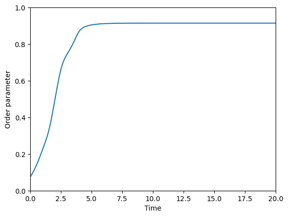
Wow, the oscillators are synchronized! The order parameter \(r\) is close to one. Let’s observe the final state of the oscillators for \(K=1.0\) and \(K=3.0\).

n_oscillator = 100

_thetas = jnp.arange(0, 2*jnp.pi, 0.01)
rx_nonsync = jnp.mean(jnp.cos(final_thetas_0))
ry_nonsync = jnp.mean(jnp.sin(final_thetas_0))
r_nonsync = jnp.sqrt(rx_nonsync**2 + ry_nonsync**2)
rx_sync = jnp.mean(jnp.cos(final_thetas_1))
ry_sync = jnp.mean(jnp.sin(final_thetas_1))
r_sync = jnp.sqrt(rx_sync**2 + ry_sync**2)

plt.figure(figsize=(10, 5))
plt.subplot(1, 2, 1)
plt.xlim(-1.1, 1.1)
plt.ylim(-1.1, 1.1)
plt.plot(jnp.cos(_thetas), jnp.sin(_thetas), color="gray", ls="dashed", zorder=0)
plt.scatter(jnp.cos(final_thetas_0), jnp.sin(final_thetas_0), s=10, zorder=10)
plt.plot([0, rx_nonsync], [0, ry_nonsync], color="gray", lw=2, zorder=20)
plt.scatter([rx_nonsync], [ry_nonsync], color="red", zorder=30)
plt.title(f"K=1.0: r={r_nonsync:.3f}")

plt.subplot(1, 2, 2)
plt.xlim(-1.1, 1.1)
plt.ylim(-1.1, 1.1)
plt.plot(jnp.cos(_thetas), jnp.sin(_thetas), color="gray", ls="dashed", zorder=0)
plt.scatter(jnp.cos(final_thetas_1), jnp.sin(final_thetas_1), s=10, zorder=10)
plt.plot([0, rx_sync], [0, ry_sync], color="gray", lw=2, zorder=20)
plt.scatter([rx_sync], [ry_sync], color="red", zorder=30)
plt.title(f"K=3.0: r={r_sync:.3f}")
plt.show()

We have been using the from-scrtach implementation of the Kuramoto model. This package, jaxkuramoto, provides the same implementation as above with few lines of code.

Use `jaxkuramoto` instead#

We introduce jaxkuramoto package, which provides the Kuramoto model and the numerical integrator. There are mainly three steps to use jaxkuramoto:

Define the distribution of the natural frequencies
Define the model
Run the simulation

Define the distribution of the natural frequencies#

In many research papers, natural frequencies \(\omega_{i}\) are chosen randomly from some distribution. jaxkuramoto provides several distributions, and also allows you to define your own distribution. If you want to use the normal distribution, you can do as follows.

from jaxkuramoto.distribution import Normal

dist = Normal(0.0, 1.0)
omegas = dist.sample(random.PRNGKey(0), (n_oscillator,))

We are also creating other distributions. Check out here for more details!!

Define the model#

Now we define the model. We have Kuramoto class, which takes the natural frequencies and the coupling strength as arguments.

from jaxkuramoto import Kuramoto

K = 3.0
model = Kuramoto(omegas, K)

Run the simulation#

Warning

Currently, we are using jaxkuramoto.odeint for integrating ODEs. This is because other ODE libraries are not supporting observable_fn option. However, diffrax, numerical differentiation library for JAX, is currently implementing this functionality and will be released in the future. We will switch to diffrax when it is released. See this issue and this pull request for more details.

That’s it! Now we can run the simulation. We can also specify the numerical integrator, the initial time, the final time, and the time step. Kuramoto class has vector_fn method, which returns the vector field of the Kuramoto model, and orderparameter method, which returns the order parameter \(r\).

from jaxkuramoto.solver import runge_kutta
from jaxkuramoto import odeint

t0, t1, dt = 0.0, 20.0, 0.01
init_thetas = random.uniform(random.PRNGKey(1), (n_oscillator,), maxval=2*jnp.pi)
sol = odeint(model.vector_fn, runge_kutta, t0, t1, dt, init_thetas, model.orderparameter)

odeint returns the solution of the ODEs, which is a Solution class. Let’s visualize the time evolution of the order parameter \(r\).

plt.xlim(0, t_max)
plt.ylim(0, 1.0)
plt.xlabel("Time")
plt.ylabel("Order parameter")
plt.plot(sol.ts, sol.observables)
plt.show()

Solution class also has a final_state attribute, which returns the final state of the system.

plt.figure(figsize=(5, 5))
plt.xlim(-1.1, 1.1)
plt.ylim(-1.1, 1.1)
plt.plot(jnp.cos(_thetas), jnp.sin(_thetas), color="gray", ls="dashed", zorder=0)
plt.scatter(jnp.cos(sol.final_state), jnp.sin(sol.final_state), s=10, zorder=10)
plt.title(f"K=3.0: r={sol.observables[-1]:.3f}")
plt.show()

Conclusion#

In this example, we have learned how to use jaxkuramoto package to simulate the Kuramoto model. I hope that this package will be useful for your research.

We have obseved that synchoronization can occur when the coupling strength \(K\) is large. In the next page, we calculate the exact value of \(r\) with respect to \(K\)!!

References#

We recommend [Str00] for the introduction to the Kuramoto model for those who are new to this topic.

Kur75: Yoshiki Kuramoto. Self-entrainment of a population of coupled non-linear oscillators. In International Symposium on Mathematical Problems in Theoretical Physics, pages 420–422. Springer-Verlag, 1975. URL: https://doi.org/10.1007/bfb0013365, doi:10.1007/bfb0013365.
Str00: Steven H. Strogatz. From Kuramoto to Crawford: exploring the onset of synchronization in populations of coupled oscillators. Physica D: Nonlinear Phenomena, 143(1-4):1–20, September 2000. URL: https://doi.org/10.1016/s0167-2789(00)00094-4, doi:10.1016/s0167-2789(00)00094-4.

jaxkuramoto reference documentation

Kuramoto model

Contents

Kuramoto model#

Governing equations#

Order parameter#

From scratch#

Use `jaxkuramoto` instead#

Define the distribution of the natural frequencies#

Define the model#

Run the simulation#

Conclusion#

References#

jaxkuramoto reference documentation

Kuramoto model

Contents

Kuramoto model#

Governing equations#

Order parameter#

From scratch#

Use jaxkuramoto instead#

Define the distribution of the natural frequencies#

Define the model#

Run the simulation#

Conclusion#

References#

Use `jaxkuramoto` instead#