List of distributions
Contents
List of distributions#
import jax; jax.config.update("jax_enable_x64", True)
import jax.numpy as jnp
from jaxkuramoto import distribution

import matplotlib.pyplot as plt

xs = jnp.arange(-5, 5, 0.01)
Matplotlib is building the font cache; this may take a moment.
No GPU/TPU found, falling back to CPU. (Set TF_CPP_MIN_LOG_LEVEL=0 and rerun for more info.)
Normal distribution#
Probability density function
parameters
\(\mu\): mean (
loc)\(\sigma\): standard deviation (
scale)
loc = 0.0
scale = 1.0

dist = distribution.Normal(loc=loc, scale=scale)
plt.plot(xs, dist.pdf(xs), label="pdf")
[<matplotlib.lines.Line2D at 0x7fbb3ff62f40>]

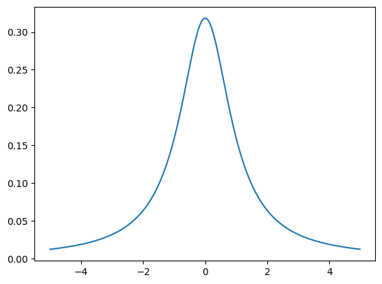
Cauchy distribution#
Probability density function
parameters
\(\mu\): location (
loc)\(\gamma\): scale (
gamma)
loc = 0.0
gamma = 1.0

dist = distribution.Cauchy(loc=loc, gamma=gamma)
plt.plot(xs, dist.pdf(xs), label="pdf")
[<matplotlib.lines.Line2D at 0x7fbb3c3ebfd0>]
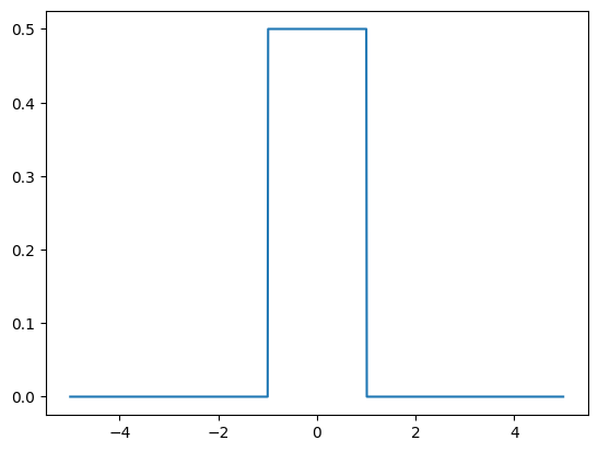
Uniform distribution#
Probability density function for \(a\leq x\leq b\)
parameters
\(a\): lower bound (
low)\(b\): upper bound (
high)
low = -1.0
high = 1.0

dist = distribution.Uniform(low=low, high=high)
plt.plot(xs, dist.pdf(xs), label="pdf")
[<matplotlib.lines.Line2D at 0x7fbb3c3a32b0>]
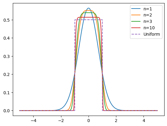
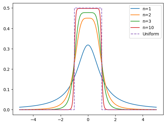
Generalized Normal distribution#
Probability density function
parameters
\(\mu\): location (
loc)\(\gamma\): scale (
gamma)\(n\): shape (
n)
Note:
\(n=1\) is the normal distribution
\(n\to\infty\) is uniform distribution (range of \(x\) is \(|x-\mu|<\gamma\))
\[ \frac{n\gamma}{\Gamma(1/(2n))}\exp(-\gamma^{2n}(x-\mu)^{2n})\to\frac{1}{2\gamma} \]
loc = 0.0
gamma = 1.0

for n in [1,2,3,10]:
    dist = distribution.GeneralNormal(loc=loc, gamma=gamma, n=n)
    plt.plot(xs, dist.pdf(xs), label=f"n={n}")
dist_uniform = distribution.Uniform(low=-gamma, high=gamma)
plt.plot(xs, dist_uniform.pdf(xs), label="Uniform", linestyle="--")
plt.legend()
<matplotlib.legend.Legend at 0x7fbb3c2b2f10>
Generalized Cauchy distribution#
Probability density function
parameters
\(\mu\): location (
loc)\(\gamma\): scale (
gamma)\(n\): shape (
n)
Note:
\(n=1\) is Cauchy distribution
\(n\to\infty\) is uniform distribution (range of \(x\) is \(|x-\mu|<\gamma\))
\[ \frac{n\sin(\pi/(2n))}{\pi}\frac{\gamma^{2n-1}}{x^{2n}+\gamma^{2n}}\to\frac{1}{2\gamma} \]
loc = 0.0
gamma = 1.0

for n in [1,2,3,10]:
    dist = distribution.GeneralCauchy(loc=loc, gamma=gamma, n=n)
    plt.plot(xs, dist.pdf(xs), label=f"n={n}")
dist_uniform = distribution.Uniform(low=-gamma, high=gamma)
plt.plot(xs, dist_uniform.pdf(xs), label="Uniform", linestyle="--")
plt.legend()
<matplotlib.legend.Legend at 0x7fbb3c2812e0>
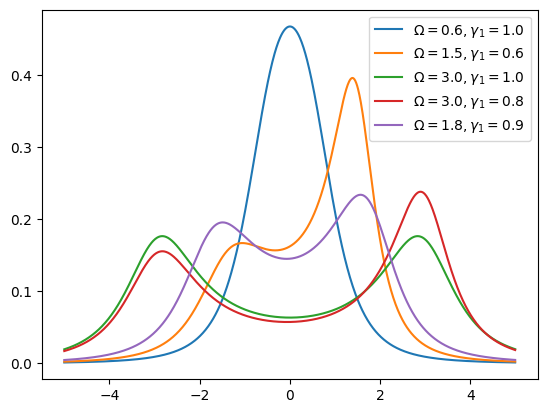
Muliplied Cauchy distribution#
Probability density function
parameters
\(\Omega\): location (
Omega)\(\gamma_{1}\): scale (
gamma1)\(\gamma_{2}\): scale (
gamma2)
# Omega, gamma1, gamma2
params = [
    (0.6, 1.0, 1.0), (1.5, 0.6, 1.0), (3.0, 1.0, 1.0),
    (3.0, 0.8, 1.0), (1.8, 0.9, 1.0)
]
for Omega, gamma1, gamma2 in params:
    dist = distribution.CauchyMultiply(Omega=Omega, gamma1=gamma1, gamma2=gamma2)
    plt.plot(xs, dist.pdf(xs), label=rf"$\Omega={Omega}, \gamma_{1}={gamma1}$")
plt.legend()
<matplotlib.legend.Legend at 0x7fbb3c1fb160>
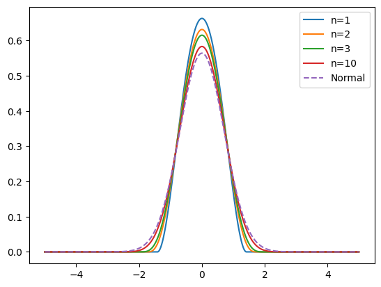
Finite-differentiable distribution#
Probability density function for \(|x-\mu|\leq\gamma\)
parameters
\(\mu\): mean (
loc)\(\gamma\): represent the scale of the distribution (
scale)
Note:
This distribution has the smoothness of \(C^{n}\) but not \(C^{n+1}\) for finite \(n\).
\(B(x, y)\) is the beta function.
By scaling \(\gamma=\sqrt{n+1}\gamma\), this distribution goes to the noraml distribution with the standard deviation \(\gamma/\sqrt{2}\) in the limit of \(n\to\infty\).
\[ \frac{1}{\sqrt{n+1}\gamma B(n+2, 1/2)}\left[1 - \frac{1}{n+1}\left(\frac{x-\mu}{\gamma}\right)^{2}\right]^{n+1}\to\frac{1}{\gamma\sqrt{\pi}}\exp\left(-\frac{(x-\mu)^{2}}{\gamma^{2}}\right) \]
loc = 0.0
gamma = 1.0
for n in [1,2,3,10]:
    scale = gamma * jnp.sqrt(n + 1)
    dist = distribution.FiniteDifferential(loc=loc, scale=scale, n=n)
    plt.plot(xs, dist.pdf(xs), label=f"n={n}")
dist_normal = distribution.Normal(loc=loc, scale=gamma / jnp.sqrt(2))
plt.plot(xs, dist_normal.pdf(xs), label="Normal", linestyle="--")
plt.legend()
<matplotlib.legend.Legend at 0x7fbb1eff3610>